IBFV for Curved Surfaces - ibfvs.exe

Introduction

The program ibfvs.exe was used to produce the images, the video and animations. We will make it publicly available if the paper is accepted for publication. The program runs under Windows'98 and higher, starting from a 350 MHz PC with TNT2 graphics. Obviously, the faster the processor and graphics board, the better the performance.

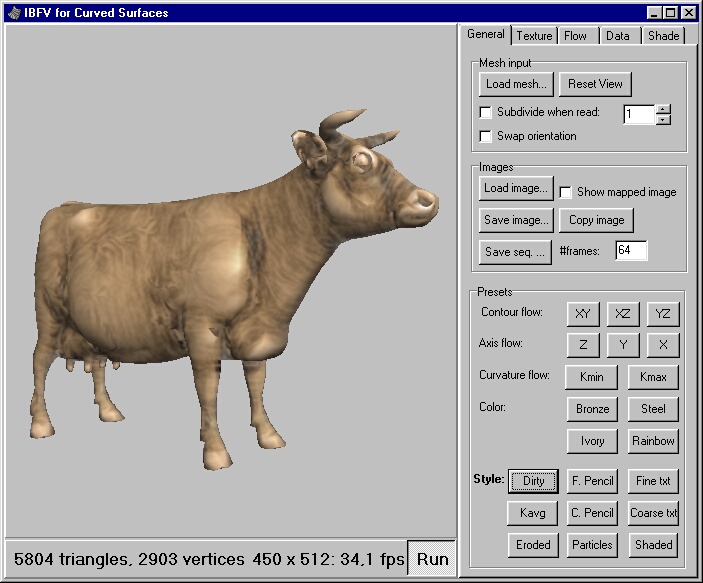
This program was developed as a prototype to experiment with different methods and techniques. For demo purposes, we have added a number of preset buttons to make a quick start. Here we will not describe all features, just give an overview of the main options such that the results shown in the paper can be reproduced.

Basics

To start ibfvs.exe, download ibfvs.zip. This archive contains the executable (ibfvs.exe) and a number of demo files. Unzip this archive, and click on the ibfvs.exe icon. An "Open file" dialog appears. In the ibfvs directory we have put a number of example files, just for review purposes. These are in the Stanford PLY format. Most of them contain only triangular meshes, in the hellerman_*deg.ply files we have also added (ad hoc) a time-dependent flow field. We know the original origin of most files, but if someone can inform us who has defined the cow and venus, we will be happy to include a reference.
The bunny originates from the Stanford 3D Scanning Repository, the Hellerman datasets were derived from data obtained from the International Research Institute for Climate Predition IRI , the other files were generated with a custom geometry generator.

Select for instance cow.ply. An ugly image appears. Press the Run button (below the image). The ugly image starts to animate. No flow field has been defined yet, so no moving texture is visible. On the right a control-panel is shown, with five tabpages. The General tabpage is the most important. Press now the Dirty button. The cow turns into dirty bronze. Try the other style buttons. Their meaning is:

Dirty: Dirty bronze: Use Kmax for modulation, flow aligned with kmin;
Kavg: Average: Use Kavg for modulation, flow aligned with kmin;
Eroded: Eroded bronze: Use Kmin for modulation, flow aligned with kmin;

F. Pencil: Fine Pencil Drawing, use shade for modulation, downward flow, turn off shading, use s = 2.0;
C. Pencil: Coarse Pencil Drawing, use shade for modulation, downward flow, turn off shading, use s = 3.0;
Particles: Moving particles over surface, adapt texture temporal pattern, switch on full (Texture panel);

Fine txt: Fine texture, use default settings, use s = 2.0;
Coarse txt: Coarse texture, use default settings, use s = 3.0;
Shaded: Show only shaded image, no texture.

Note that only the first five buttons define a flow field, the particles and moving textures use the current flow field.
Also for the flow field preset buttons are available in the General tabpage:

along contours (XY, XZ, YZ plane),
along axes (Z, Y, X), and
along principal directions (Kmin and Kmax).

These buttons control the settings in the Flow tabpage. Furthermore, some colors can be set from the General tabpage.

Changing the view can be done simply with the mouse. Put the cursor in the image,
press:

the left button for rotation,
the middle button for translation, and
the right button for scaling;

and drag the mouse. If a default view is desired (often after reading in a new file), press Reset View (General tabpage).

The quality of the results can be improved strongly by using a more fine and smooth mesh. To this end, enable the Subdivide when read checkbox (General tabpage), select a subdivision level (1-4), press Load mesh... and reread the current ply file or read in a new one. Beware that the number of polygons depends exponentially on the subdivision level... We typically use 1-2 for the cow, 2-3 for the torso, and 0 for the bunny.

With this, it should be possible to reproduce figure 9, 10, and 11 of the paper. For curvature flow the results can be improved sometimes by selecting a different alignment of the flow. For this, go to the Flow tabpage, and press the Align X, Y, or Z buttons. To produce the other examples, the following can be done.

Special effects

For the flow on the earth (figure 6), the safest is first to restart the program, such that all values have their defaults. Load hellerman_2deg.ply or hellerman_4deg.ply, without subdivision. The first has a resolution of two degrees, the second of four degrees. Press Run. In the General tabpage, press Load image... and select worldmap512.bmp. To show the magnitude of the flow:

On the Data tabpage: Set the Max (imum) range of the data to 2 (followed by <Enter>) and turn on Overlay with data.
On the Texture tabpage: Disable Scale up to maximum displacement and enable Modulate alpha for data.
To see the worldmap again, disable Overlay with data (Data tabpage).
Time dependent data can be shown by entering a time step dt (followed by <Enter>) in the Data tabpage. The unit is a month, 0.1 gives a good result, and enable the animate checkbox.

For topology flow (figure 7), start from scratch again to be safe, and load either bsurf.ply or bsurf_big.ply. Next:

Press Run;
Press Axis flow Y (General tabpage);
Select a top view on the surface with the mouse;
Press the Topology button on the Texture tabpage;
Wait a few seconds until the image stabilizes;
Enable Lock texture;
Drag the surface around;
Disable Lock texture again.

This produces valley lines. To get ridge lines, use the same steps, but after Axis flow Y, go to the Flow tabpage, and set Angle to 180 degrees.

To produce user defined flow (figure 5), load a geometry (for instance the cow) and press Run. Switch to the Flow tabpage. A linear flow field can be defined with the three values behind Linear. To add a flow source, press Add flow. Line sources can be dragged interactively, either via the end-points or via the cylinder. Motion is constrained to a plane, rotate the object to activate another plane. Note that line sources extend infinitely. The flow strength can be set with the three items Strength (attract, repulse), Rotational (around the line), and Tangential (along the line).
For a more colorful picture, go to the Data tabpage, and enable Overlay with data (with Velocity selected). Adapt the range Min-Max if needed, either by entering values, or with the >, <, <>, and >< buttons.

If other PLY files are read and strange results appear, the following can be tried. Enable Swap orientation (General tabpage) and reread the file. The orientation of all triangles is reversed, hence front side turns into far side Furthermore, by default we assume that the Z-axis points to the viewer and the Y-axis up. This can be changed on the Shade tabpage by selecting a different Up axis..

Technical aspects

Concerning technical details discussed in section 3, a few hints to see them alive. For all, start the program, load the cow, select Axis flow Y, and press Run.

3.4 Contrast. The balance between texture and shading can be varied with the parameter Alpha shade on the Texture tabpage. The number gives the percentage of shading to be used (i.e. reverse of beta in the paper). A value of 0 gives an image of Ft, a value of 100 gives Fs.

3.5 Boundaries and silhouettes. The background color can be changed on the Shade tabpage. Press the grey rectangle behind Background, select bright red, and see what happens. The effect depends strongly on the value of alpha. This can be set on the Texture tabpage (Alpha texture). Change it for instance in unit steps from 0 to 20 to see the effect. For values higher than 5 (= 0.05), the inflow of red ink decreases rapidly.

3.7 Projected texture. By default we use the mode to drag the textures Ft and G along with the mouse. To see the effect, disable Drag texture when changing view on the Texture tabpage. Especially for panning (middle mouse button) the effect is strong: Now the texture appears to stick to the screen. Also, locking can be enabled and disabled with the two checkboxes Lock texture and Lock texture when changing view.

3.8 Non surface-aligned flow. By default, velocities are projected on the surface. This can be disabled with the checkbox Project velocity on surface on the Flow tabpage.

3.9 Texture interpolation. Zoom in on a side of the cow. At some point, the stationary flow gets distorted in a strange way, the closer, the stronger. The mesh can be shown by enabling the Mesh checkbox in the Shade tabpage. The weird patterns are related to the mesh. Next, enable isometric in the Shade tabpage. The strange patterns disappear.
(The clipping planes are set in a slightly different way for isometric mode. Hence, recentering can be necessary. Also, the depth shift for the mesh is not implemented full proof :-) ). Another way to get rid of the texture interpolation artifact is by using extra subdivision, leading to smaller triangles.