A knot is a simple closed curve (homeomorphic image of S(1)) in Euclidean 3-space E(3). Two knots are called equivalent when there is an orientation-preserving homeomorphism of E(3) onto itself sending one knot to the other.
Schoenflies proved in 1908 that any homeomorphism from a simple closed curve in the plane E(2) onto the unit circle S(1) can be extended to a homeomorphism of the plane onto itself. Similar things do not hold in higher dimensions.
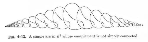
For example, there exist wild embeddings of simple arcs into E(3): homeomorphic images of the unit interval such that the complement is not simply connected. Thus, one usually restricts knots to be tamely embedded, e.g., as a simple closed polygonal curve, and we'll do so as well.
Two more examples of wild embeddings:
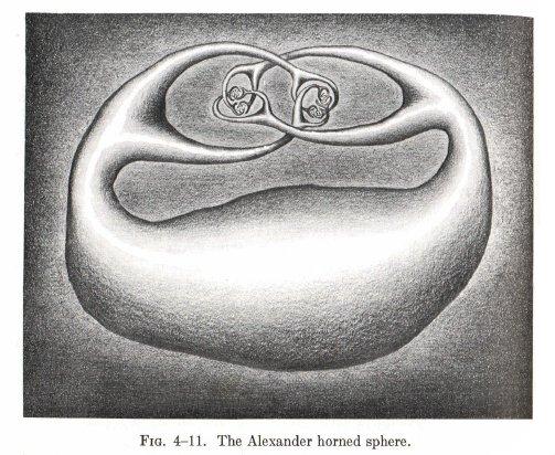
Example (Alexander's horned sphere) A homeomorphic image of the sphere S(2) in E(3) such that the complement of the image is not simply connected.
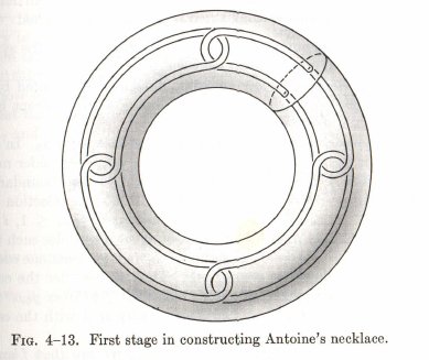
Example (Antoine's necklace) A homeomorphic image of the Cantor set (which is compact and totally disconnected) in E(3) such that the complement of the image is not simply connected.
(The pictures here were taken from Hocking & Young, Topology, pp. 176-177.)
Given a knot in E(3), we project it from a point in general position into E(2), so that the resulting curve never passes three times through the same point, and indicate for each crossing whether it is an over- or undercrossing. The resulting diagram suffices to retrieve the knot up to equivalence.
Now equivalence between knots can be translated into equivalence between diagrams. This was done by Reidemeister, who showed that two diagrams represent the same knot if and only if one is obtained from the other by a sequence of Reidemeister moves:
in each of the three types of move, we may replace the upper picture by the lower, or vice versa; type I also has a mirror image, type I'.
There is a unique knot with a diagram without crossings: the unknot.
There is a composition of knots: roughly: tying one after the other. One takes two oriented knots, places two straight line segments with opposite orientation on top of each other, making them cancel. The resulting knot is uniquely determined by the two knots one started with. A knot is called prime if it is not the sum (defined in this way) of two knots, both different from the unknot. Of course this is precisely the 1-dimensional analogue of the # glueing operation used in the previous section.
(This picture was taken from Lickorish, An Introduction to Knot Theory, p. 6.)
Note that the unknot is a zero element for this sum operation. We have a unique `prime factorization': each knot is a sum of a finite number of prime knots, and the prime knots that go into a knot are uniquely determined.
This can be proved by associating a Seifert surface to the knot. A Seifert surface of a link is a compact oriented surface in S(3) with the given link as boundary. Every link has a Seifert surface: give the link some orientation, take a diagram, and replace each crossing by a non-crossing by making the upper strand turn left. Now the diagram has become a union of circuits and we can pick disjoint discs with these circuits as boundaries. Now for each crossing that we replaced, insert a half-twisted strip joining the discs. This yields an oriented surface with the original link as boundary.
Now one can define the genus of a knot as the minimal genus of a Seifert surface Ffor it. (Where one might define the genus in this case by g = (1 - chi(F))/2 where chi(F) is the Euler characteristic. The genus is additive: g(K1 + K2) = g(K1) + g(K2), and is nonnegative, and is zero only for the unknot. It follows that the sum of two knots can only be the unknot when both knots are the unknot themselves.
The Seifert surface of a knot is orientable and has a single boundary component, so g = (1 - chi(F))/2 = h is the number of handles, a nonnegative integer, and zero precisely for the unknot.
Pictures of the prime knots with a plane drawing with at most 8 crossings (after G. Burde, `Knoten', Jahrbuch Ueberblicke Mathematik, B.I. Mannheim, 1978, pp. 131-147 which contains drawings of the knots with at most 9 crossings. A table of the knots with at most 10 crossings is found in D. Rolfsen, `Knots and Links', Publish or Perish, 1976). The unknot is omitted and orientation is disregarded.


All except the last three are alternating: they have a diagram where along the knot overcrossings and undercrossings alternate.
One of the objects of knot theory is to distinguish inequivalent knots. To this end many invariants have been invented. In this context the most obvious invariant of a knot K is the fundamental group of its complement E(3) \ K.
A complete invariant is the complement itself as a topological space: C. Gordon and J. Luecke, `Knots are Determined by their Complements', J. Amer. Math. Soc. 2, 371-415, 1989.
Kauffman defines a Laurent polynomial in a variable A (i.e., a polynomial in A and A^(-1)) for each unoriented link diagram D in S(2) as follows: If D is a simple loop, then <D> = 1. If D is the disjoint union of D' and a simple loop, then <D> = (-A^2-A^(-2))<D'>. Otherwise, pick a crossing in D and make diagrams D' and D'' by replacing the crossing by two turns where the upper strand turns left in D' and right in D''. Now define <D> = A <D'> + A^(-1)<D''>.
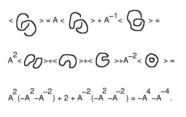
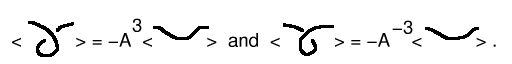
Then (1) the Kauffman bracket is well-defined, i.e., does not depend on the order in which crossings are eliminated, and (2) the Kauffman bracket is invariant for Reidemeister moves of types II and III. It is not invariant for Reidemeister moves of type I. Indeed, we find
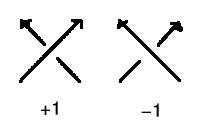
Now given an oriented link we can do a bit more, and distinguish two types of crossing: those where the top comes from the left (+1) and those where the top comes from the right (-1). Adding the values for all crossings we get the writhe of the diagram. For an unoriented knot this is defined too: the sign of a crossing does not change when the orientation is reversed.
The Jones polynomial V(L) of a link L is defined by V(L) = ((-A)^(-3w) <D>) where D is any oriented diagram of L and w is the writhe of D. The usual variable in V(L) is t, where t = A^(-4). Now V(L) is a polynomial in t when the number of components of L is odd, and in particular when L is a knot.
A link is a disjoint union of simple closed curves in E(3). Thus, each connected component is a knot, and these knots may be entangled. The smallest few examples are shown here.


(Two links can be nonequivalent but have homeomorphic complements, see C.C. Adams, `The Knot Book: An Elementary Introduction to the Mathematical Theory of Knots', W. H. Freeman, New York, pp. 280-286, 1994.)
A link is trivial if and only if the fundamental group of the complement is free.
A braid on n strings is a collection of n arcs in E(3) starting at the n points (0,j,1) and ending at the n points (0,j,0), j = 1,2,...,n, each meeting the planes z = c (with 0 < c < 1) in a unique point.
The elementary braid s(i) is the braid interchanging the two strands numbered i and i+1, where the former overcrosses the latter, where all other strands go straight from top to bottom.
We have the obvious concept of composition of braids (similar to that of composition of paths), and find that every braid is (equivalent to) the product of elementary braids.
The braid group B(n) of braids with n strings is isomorphic to the group with generators s(i) (i=1,...,n-1) and relations (i) s(i) s(j) = s(j) s(i) when |i-j| > 1, and (ii) s(i) s(i+1) s(i) = s(i+1) s(i) s(i+1) for all i. (Artin)
It is possible to view B(n) as the fundamental group of a topological space. (Fox)
A theorem by Alexander (J.W. Alexander, `A lemma on systems of knotted curves', Proc. Nat. Acad. Sci. USA 9 (1923) 93-95) shows that every link is equivalent to one obtained from a braid by identifying starting and ending points.