The toolchain
Installation instructions
There are two distributions available for download (source and binary):
- binary distribution
- Download the binary archive from the download page.
- Unpack the archive into a directory of choice.
- Invoke the tools from the commandline like this:
<tool-name> <parameter>
- source distribution
- If no recent version of python is installed on your system, go to www.python.org and download the latest python version (beware, python 3.x is not supported at this time). The compiler, loader and simulator have been implemented and tested in python version 2.5.1.
- Download the source archive from the download page.
- Unpack the source archive into a directory of choice.
- Make sure that all files in the dependencies directory are placed on the pythonpath (e.g. <Python installdir>\Lib\site-packages).
- Invoke the tools from the commandline like this:
python <sourcefile> <parameters>
Overview
The toolchain consists of four main programs:
- a compiler
- a loader
- a simulator
- a bridge
The following figure shows how they toolchain and sensor networks work together.
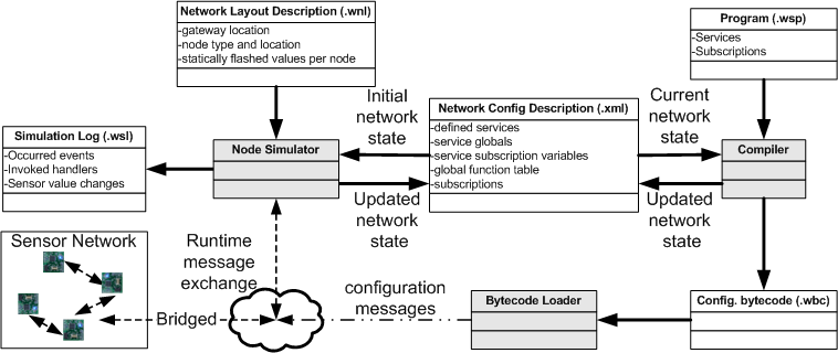
Files:
- .wsp: a high-level network program (specifies entire network behaviour)
- .wbc: configuration messages with embedded bytecode
- .xml: symbol table of the compiler (reflects network configuration)
- .wnl: layout of the simulated network (scenario description)
- .wsl: simulation log file.
Programming a sensor network with our programming model is done in four stages. First, one must generate the propert network configuration file. To do this, write a layout file for your scenario (refer to the tutorial to see how) start and then stop the simulator. This generates the initial configuration for your scenario.
The second step consists of writing a program to define and compose services. This program is passed into the compiler to generate bytecode. The compiler reads and updates the configuration file which was generated in the first step. The configuration file basically maps names of system calls, services, subscriptions, handlers, events and variables onto short IDs for efficiency and compactness considerations.
Next, the loader takes the configuration message bytecode (.wbc) as input. The loader uploads the messages to the simulator and/or the bridge application (they are broadcasted over UDP to 127.255.255.255, adjust your firewall to allow this).
Finally in the fourth stage, sensors and simulated nodes exchange messages according to the services defined in the .wsp program.
To enable hardware nodes from receiving the messages uploaded by the loader, the bridge application (serial_WASP.exe) needs to be run. This application requires installation of cygwin.
One of the hardware nodes needs to be flashed with the bridge firmware and attached your pc or laptop using a USB programmer. Next the serial_WASP.exe bridge application needs to be started. The typical command line is:
./serial_WASP serial_in logfile.bin serial_out
where serial_in and serial_out refer to the serial port where a node is attached (like /dev/com7) and both are typically the same. The logfile.bin file is used to log serial traffic, for debugging or replaying.
The application is further configured with environment variables (this will be improved).
| variable | description | default |
|---|---|---|
| OSAS_SIM_PORT | UDP base port for the simulation | 5500 |
| OSAS_SIM_SEND_ADDRESS | UDP address to send data, | 127.255.255.255 |
| OSAS_SIM_RECV_ADDRESS | UDP address to listen to data, | 127.0.0.1 |
| OSAS_WASP_PROTOCOL | Identifier of network protocol as used within WASP | 6 (use MantisMAC through simple NWK API) |
| OSAS_DEBUG | Level of debug messages, | 0 |
| OSAS_XPOS | x position of node within the simulation | 0 |
| OSAS_YPOS | y position of node within the simulation | 0 |
| OSAS_STRENGTH | transmission strength within the simulation | 4 |
Together, OSAS_XPOS and OSAS_YPOS define the identify of a node by OSAS_XPOS*16+OSAS_YPOS. This identity (ID) should match the identity of the base station node that is attached to the serial port and the identity of the simulated node.
serial_WASP.exe will listen to port OSAS_SIM_PORT+ID+1000 for packets that need to be transmitted over the serial line. These packets should contain the destination in the header. Packets that are received over the serial line will be send to port OSAS_SIM_PORT+ID.
For example, to connect simulated node 31 (id derived from position x=1,y=15) to hardware bridge node 31 (id needs to be set to 31 in firmware) launch serial_WASP.exe like this: (adjust /dev/com4 to the correct port)
OSAS_XPOS=1 OSAS_YPOS=15 OSAS_STRENGTH=4 ./serial_WASP.exe /dev/com4 logfile.bin /dev/com4
Scenario description files
The scenario description files are an input to the simulator to describe which nodes are present in the scenario, what their location is (currently, stationary) and what the contents of Ncontext are for each node.
The scenario description for the simulator has the following grammar:
PARAM ::= <python datatype>
PARAMS ::= PARAM {' ' PARAMS}
ENTRY ::= integer integer identifier identifier PARAMS '\n'
An entry starts with an x and y coordinate of a node. Next an identifier specifies a python unit containing Subclasses of the Node class defined by the simulator. The unit identifier is followed by the name of the class to instantiate and a space separated list of (simple) python datatypes which are passed as parameter in the instantiation of the node.
The subclasses of Node can define specific node types which each have their own Ncontext (e.g. a temperature sensor would expose a function for accessing temperature readings). To see how to define your own nodetypes, refer to one of the example scenarios.